
Modeling the Prices of Homes
In this post I use information about homes sold from 2006-2010 in Ames, Iowa, to create a model for predicting sale prices, and submit my model to a Kaggle competition.
The data - which was originally published by Dean De Cock, a professor at Truman State University - has 80 variables describing the quality of homes. The data was collected by the City of Ames for purposes of tax assessment, and contains information about which one would expect potential property buyers to care, so it makes sense that it would influence price.
As of May 2018, De Cock’s 2011 publication in the Journal of Statistics Education, 19(3) can be found here: https://ww2.amstat.org/publications/jse/v19n3/decock.pdf
import pandas as pd
import matplotlib.pyplot as plt
import matplotlib
import numpy as np
import seaborn as sns

from sklearn.linear_model import RidgeCV, LassoCV, ElasticNetCV
from sklearn.model_selection import cross_val_score, train_test_split
from sklearn.preprocessing import PolynomialFeatures, StandardScaler

from sklearn.pipeline import Pipeline
from sklearn.preprocessing import StandardScaler
from sklearn.model_selection import GridSearchCV
from sklearn.metrics import r2_score

%config InlineBackend.figure_format = 'retina'
%matplotlib inline
After importing the necessary modules, I read the data from two csv files, ‘test.csv’ and ‘train.csv’
test = pd.read_csv('test.csv')
train = pd.read_csv('train.csv')
I started my exploratory data analysis by finding out how many rows and columns there are in the test and train sets.
As seen in the output of the following two cells, the training data has more rows (observations) than the test data, and also has one more column than the test data. Upon further investigation, this column is ‘price’, the target variable. This makes sense since my objective is to predict price. My predictions for price will go in the price column of the test data.
test.shape
(879, 80)
train.shape
(2051, 81)
Next I visually inspected the first few rows of each data set.
train.head()
| Id | PID | MS SubClass | MS Zoning | Lot Frontage | Lot Area | Street | Alley | Lot Shape | Land Contour | ... | Screen Porch | Pool Area | Pool QC | Fence | Misc Feature | Misc Val | Mo Sold | Yr Sold | Sale Type | SalePrice | |
|---|---|---|---|---|---|---|---|---|---|---|---|---|---|---|---|---|---|---|---|---|---|
| 0 | 109 | 533352170 | 60 | RL | NaN | 13517 | Pave | NaN | IR1 | Lvl | ... | 0 | 0 | NaN | NaN | NaN | 0 | 3 | 2010 | WD | 130500 |
| 1 | 544 | 531379050 | 60 | RL | 43.0 | 11492 | Pave | NaN | IR1 | Lvl | ... | 0 | 0 | NaN | NaN | NaN | 0 | 4 | 2009 | WD | 220000 |
| 2 | 153 | 535304180 | 20 | RL | 68.0 | 7922 | Pave | NaN | Reg | Lvl | ... | 0 | 0 | NaN | NaN | NaN | 0 | 1 | 2010 | WD | 109000 |
| 3 | 318 | 916386060 | 60 | RL | 73.0 | 9802 | Pave | NaN | Reg | Lvl | ... | 0 | 0 | NaN | NaN | NaN | 0 | 4 | 2010 | WD | 174000 |
| 4 | 255 | 906425045 | 50 | RL | 82.0 | 14235 | Pave | NaN | IR1 | Lvl | ... | 0 | 0 | NaN | NaN | NaN | 0 | 3 | 2010 | WD | 138500 |
5 rows × 81 columns
test.head()
| Id | PID | MS SubClass | MS Zoning | Lot Frontage | Lot Area | Street | Alley | Lot Shape | Land Contour | ... | 3Ssn Porch | Screen Porch | Pool Area | Pool QC | Fence | Misc Feature | Misc Val | Mo Sold | Yr Sold | Sale Type | |
|---|---|---|---|---|---|---|---|---|---|---|---|---|---|---|---|---|---|---|---|---|---|
| 0 | 2658 | 902301120 | 190 | RM | 69.0 | 9142 | Pave | Grvl | Reg | Lvl | ... | 0 | 0 | 0 | NaN | NaN | NaN | 0 | 4 | 2006 | WD |
| 1 | 2718 | 905108090 | 90 | RL | NaN | 9662 | Pave | NaN | IR1 | Lvl | ... | 0 | 0 | 0 | NaN | NaN | NaN | 0 | 8 | 2006 | WD |
| 2 | 2414 | 528218130 | 60 | RL | 58.0 | 17104 | Pave | NaN | IR1 | Lvl | ... | 0 | 0 | 0 | NaN | NaN | NaN | 0 | 9 | 2006 | New |
| 3 | 1989 | 902207150 | 30 | RM | 60.0 | 8520 | Pave | NaN | Reg | Lvl | ... | 0 | 0 | 0 | NaN | NaN | NaN | 0 | 7 | 2007 | WD |
| 4 | 625 | 535105100 | 20 | RL | NaN | 9500 | Pave | NaN | IR1 | Lvl | ... | 0 | 185 | 0 | NaN | NaN | NaN | 0 | 7 | 2009 | WD |
5 rows × 80 columns
I also opened the data in a spreadsheet program for a more thorough visual inspection of the data (since the .head() method does not show all columns). This revealed that many of the columns had missing values (as white space). In order to use these variables for modeling without getting errors, I turned these missing values into np.NaN.
# This use of the DataFrame.replace() method uses a regular expression
# to replace cells which only contain whitespace with np.NaN.
# Credit for this implementation goes to Stack Overflow user Temak
# on this thread: https://stackoverflow.com/questions/13445241/replacing-blank-values-white-space-with-nan-in-pandas

train.replace(r'^\s+$', np.nan, regex=True, inplace=True)
test.replace(r'^\s+$', np.nan, regex=True, inplace=True)
Many of the column titles have spaces, which I converted to underscores in the next cell because spaces do not play nicely with the other objects.
train.columns = [col.strip().replace(' ', '_') for col in train.columns]
test.columns =  [col.strip().replace(' ', '_') for col in test.columns]
Next I plotted the distribution of the variable of most interest, the prediction target: SalePrice.
As seen in the graph below, it has a right skewed distribution with some large outliers.
sns.distplot(train.SalePrice);
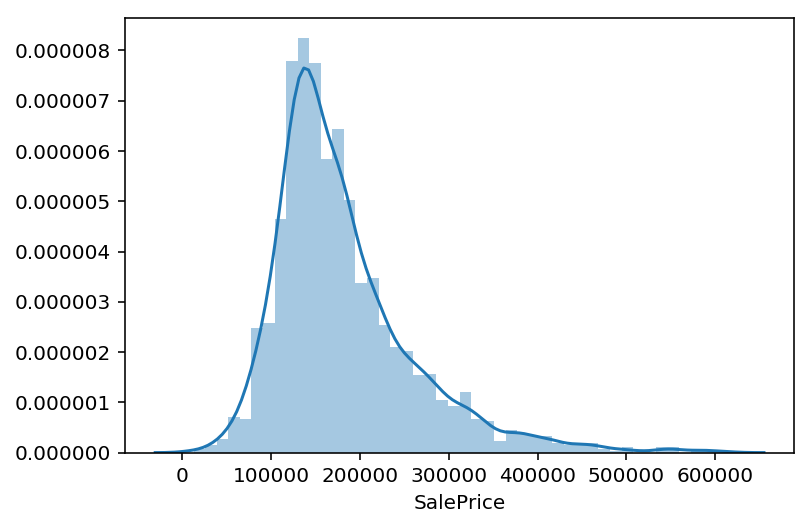
To understand the distribution of SalePrice more precisely, I used the .describe() method to get summary statistics. In dollars, the mean sale price was ~181,000, the maximum sale price was ~611,000, the minimum was ~13,000, and the middle 50% of sale prices were between ~130,000 and ~214,000.
train.SalePrice.describe()
count      2051.000000
mean     181469.701609
std       79258.659352
min       12789.000000
25%      129825.000000
50%      162500.000000
75%      214000.000000
max      611657.000000
Name: SalePrice, dtype: float64
I wish houses were this cheap in New York or Vancouver.
The date of sale could also have a lot to do with the prices, so I looked at that next.
Plotting sale frequency by month:
# This graph was inspired by Lee Clemmer's blog post here: https://www.kaggle.com/leeclemmer/exploratory-data-analysis-of-housing-in-ames-iowa/code
train.groupby(['Yr_Sold','Mo_Sold']).Id.count().plot(kind='bar',fontsize=14,figsize=(15,5),color='b')
plt.title("Amount of Sales Per Month")
plt.xlabel('Year, Month')
plt.show()
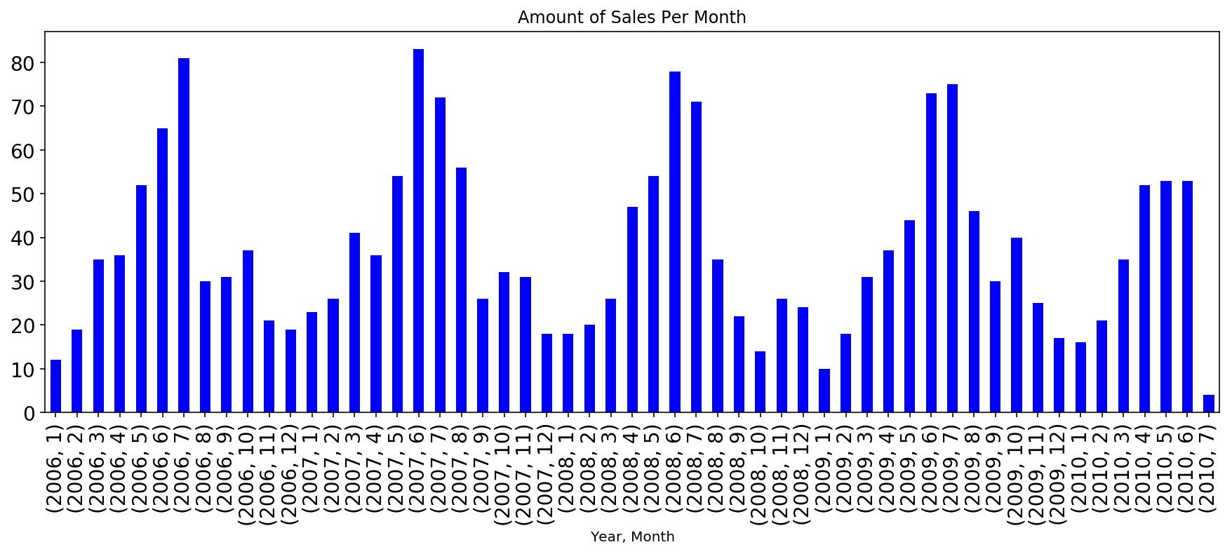
Sale dates appear seasonal, and the time period includes the ‘08 housing bubble crash. To check whether the national housing market had a notable impact on Ames house prices, I plotted sale prices by time and looked for a dip starting in 2008.
train.groupby(['Yr_Sold','Mo_Sold'])['SalePrice'].mean().plot(kind=
                                                              'bar',color='b',
                                                              figsize=(15,5));
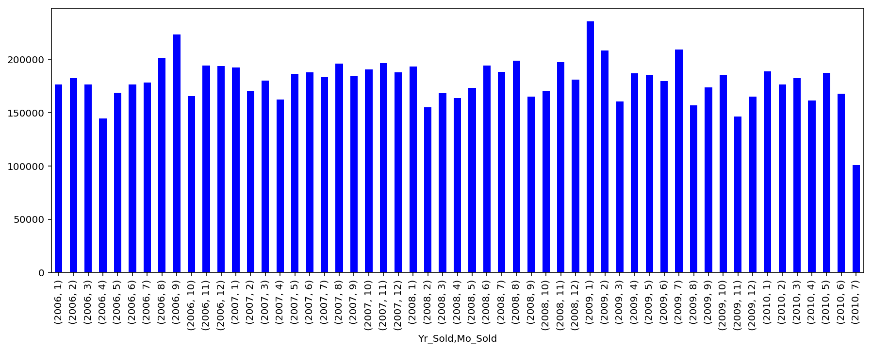
If the housing crisis impacted sale prices in Ames, the effect wasn’t drastic. However, it appears that prices tended to be lower after December of 2007 than before. This is a topic worthy of further study, though I decided not to make a variable representing when a sale happened in relation to the bubble, since any information offered by such a variable was already contained within existing variables about date of sale.
In preparation for predicting SalePrice using regularized linear regression, I log transformed SalePrice to reduce its skew and handle its large outliers. Log transforming target data is one method for handling these outliers (which the author of the dataset even recommended removing), and making cheap and expensive housing prices influence the model equally
(as argued by by Julien Cohen Solal in his analysis of the Ames data: https://www.kaggle.com/juliencs/a-study-on-regression-applied-to-the-ames-dataset/code).
# Log-transform SalePrice, the target.
train.SalePrice = np.log(train.SalePrice)
Next I continued my preparation for linear regression by making dummy variables out of the categorical and ordinal variables.
# Make dummy variables for all variables of type object, plus MS SubClass
# which, while not currently encoded as an object, still represents a categorical variable.
# Credit for this function goes to Joe Dorfman from my DSI cohort
def get_dummied(train, test):
    list = ['MS_SubClass']
    for i in train.columns:
        if train[i].dtype == object:
            list.append(i)

    full_data = pd.concat([train, test], axis = 0)
    full_data = pd.get_dummies(full_data, columns=list, drop_first = True)

    X_dummied = full_data[:len(train)]
    test_dummied = full_data[len(train):]

    return X_dummied, test_dummied

train, test = get_dummied(train, test)
# review the columns to check that get_dummied really made the dummies
train.head()
test.head()
| 1st_Flr_SF | 2nd_Flr_SF | 3Ssn_Porch | Bedroom_AbvGr | BsmtFin_SF_1 | BsmtFin_SF_2 | Bsmt_Full_Bath | Bsmt_Half_Bath | Bsmt_Unf_SF | Enclosed_Porch | ... | Misc_Feature_TenC | Sale_Type_CWD | Sale_Type_Con | Sale_Type_ConLD | Sale_Type_ConLI | Sale_Type_ConLw | Sale_Type_New | Sale_Type_Oth | Sale_Type_VWD | Sale_Type_WD | |
|---|---|---|---|---|---|---|---|---|---|---|---|---|---|---|---|---|---|---|---|---|---|
| 0 | 908 | 1020 | 0 | 4 | 0.0 | 0.0 | 0.0 | 0.0 | 1020.0 | 112 | ... | 0 | 0 | 0 | 0 | 0 | 0 | 0 | 0 | 0 | 1 |
| 1 | 1967 | 0 | 0 | 6 | 0.0 | 0.0 | 0.0 | 0.0 | 1967.0 | 0 | ... | 0 | 0 | 0 | 0 | 0 | 0 | 0 | 0 | 0 | 1 |
| 2 | 664 | 832 | 0 | 3 | 554.0 | 0.0 | 1.0 | 0.0 | 100.0 | 0 | ... | 0 | 0 | 0 | 0 | 0 | 0 | 1 | 0 | 0 | 0 |
| 3 | 968 | 0 | 0 | 2 | 0.0 | 0.0 | 0.0 | 0.0 | 968.0 | 184 | ... | 0 | 0 | 0 | 0 | 0 | 0 | 0 | 0 | 0 | 1 |
| 4 | 1394 | 0 | 0 | 3 | 609.0 | 0.0 | 1.0 | 0.0 | 785.0 | 0 | ... | 0 | 0 | 0 | 0 | 0 | 0 | 0 | 0 | 0 | 1 |
5 rows × 273 columns
Next, I added 2nd degree polynomial features for the 10 most important variables (ranked by correlation with SalePrice). I chose not to make polynomial features for all variables in order to reduce the processing time that would be required in later steps to ensure that I would have time to test multiple models.
# Assess which variables are most correlated with sale price:
corr = train.corrwith(train.SalePrice)
print(corr.sort_values(ascending=False).head(11))
SalePrice         1.000000
Overall_Qual      0.822774
Gr_Liv_Area       0.687774
Garage_Cars       0.667780
Garage_Area       0.650755
Year_Built        0.624449
Total_Bsmt_SF     0.621416
Year_Remod/Add    0.599459
1st_Flr_SF        0.599086
Garage_Yr_Blt     0.581093
Full_Bath         0.565855
dtype: float64
# Make a list of the columns to be passed to PolynomialFeatures()
cols = ['Overall_Qual','Gr_Liv_Area','Garage_Cars','Garage_Area',
        'Year_Built','Total_Bsmt_SF','Year_Remod/Add', '1st_Flr_SF',
        'Garage_Yr_Blt','Full_Bath']

# Instantiate PolynomialFeatures with intercept = False
poly = PolynomialFeatures(include_bias=False)

# Make 2nd degree polynomials from the variables in cols
# Filling all NaNs with 0s because you can't multiply times a NaN
# And turn them back into dataframes
train_poly = pd.DataFrame(poly.fit_transform(train[cols].fillna(0)))
test_poly = pd.DataFrame(poly.fit_transform(test[cols].fillna(0)))

# I don't care about the column names because I'm not trying to make an
# inferential model, just a predictive one
# check that the features of both dataframes line up
test_poly.head()
train_poly.head()
| 0 | 1 | 2 | 3 | 4 | 5 | 6 | 7 | 8 | 9 | ... | 55 | 56 | 57 | 58 | 59 | 60 | 61 | 62 | 63 | 64 | |
|---|---|---|---|---|---|---|---|---|---|---|---|---|---|---|---|---|---|---|---|---|---|
| 0 | 6.0 | 1479.0 | 2.0 | 475.0 | 1976.0 | 725.0 | 2005.0 | 725.0 | 1976.0 | 2.0 | ... | 4020025.0 | 1453625.0 | 3961880.0 | 4010.0 | 525625.0 | 1432600.0 | 1450.0 | 3904576.0 | 3952.0 | 4.0 |
| 1 | 7.0 | 2122.0 | 2.0 | 559.0 | 1996.0 | 913.0 | 1997.0 | 913.0 | 1997.0 | 2.0 | ... | 3988009.0 | 1823261.0 | 3988009.0 | 3994.0 | 833569.0 | 1823261.0 | 1826.0 | 3988009.0 | 3994.0 | 4.0 |
| 2 | 5.0 | 1057.0 | 1.0 | 246.0 | 1953.0 | 1057.0 | 2007.0 | 1057.0 | 1953.0 | 1.0 | ... | 4028049.0 | 2121399.0 | 3919671.0 | 2007.0 | 1117249.0 | 2064321.0 | 1057.0 | 3814209.0 | 1953.0 | 1.0 |
| 3 | 5.0 | 1444.0 | 2.0 | 400.0 | 2006.0 | 384.0 | 2007.0 | 744.0 | 2007.0 | 2.0 | ... | 4028049.0 | 1493208.0 | 4028049.0 | 4014.0 | 553536.0 | 1493208.0 | 1488.0 | 4028049.0 | 4014.0 | 4.0 |
| 4 | 6.0 | 1445.0 | 2.0 | 484.0 | 1900.0 | 676.0 | 1993.0 | 831.0 | 1957.0 | 2.0 | ... | 3972049.0 | 1656183.0 | 3900301.0 | 3986.0 | 690561.0 | 1626267.0 | 1662.0 | 3829849.0 | 3914.0 | 4.0 |
5 rows × 65 columns
# concatonate the new polynomial features with the existing X features
X_test = pd.concat([test, test_poly], axis=1)
X_train = pd.concat([train, test_poly], axis=1)

# check the result of the concatonation
X_train.head()
X_test.head()
| 1st_Flr_SF | 2nd_Flr_SF | 3Ssn_Porch | Bedroom_AbvGr | BsmtFin_SF_1 | BsmtFin_SF_2 | Bsmt_Full_Bath | Bsmt_Half_Bath | Bsmt_Unf_SF | Enclosed_Porch | ... | 55 | 56 | 57 | 58 | 59 | 60 | 61 | 62 | 63 | 64 | |
|---|---|---|---|---|---|---|---|---|---|---|---|---|---|---|---|---|---|---|---|---|---|
| 0 | 908 | 1020 | 0 | 4 | 0.0 | 0.0 | 0.0 | 0.0 | 1020.0 | 112 | ... | 3802500.0 | 1770600.0 | 3724500.0 | 3900.0 | 824464.0 | 1734280.0 | 1816.0 | 3648100.0 | 3820.0 | 4.0 |
| 1 | 1967 | 0 | 0 | 6 | 0.0 | 0.0 | 0.0 | 0.0 | 1967.0 | 0 | ... | 3908529.0 | 3888759.0 | 3908529.0 | 3954.0 | 3869089.0 | 3888759.0 | 3934.0 | 3908529.0 | 3954.0 | 4.0 |
| 2 | 664 | 832 | 0 | 3 | 554.0 | 0.0 | 1.0 | 0.0 | 100.0 | 0 | ... | 4024036.0 | 1331984.0 | 4024036.0 | 4012.0 | 440896.0 | 1331984.0 | 1328.0 | 4024036.0 | 4012.0 | 4.0 |
| 3 | 968 | 0 | 0 | 2 | 0.0 | 0.0 | 0.0 | 0.0 | 968.0 | 184 | ... | 4024036.0 | 1941808.0 | 3881610.0 | 2006.0 | 937024.0 | 1873080.0 | 968.0 | 3744225.0 | 1935.0 | 1.0 |
| 4 | 1394 | 0 | 0 | 3 | 609.0 | 0.0 | 1.0 | 0.0 | 785.0 | 0 | ... | 3853369.0 | 2736422.0 | 3853369.0 | 1963.0 | 1943236.0 | 2736422.0 | 1394.0 | 3853369.0 | 1963.0 | 1.0 |
5 rows × 338 columns
Continuing to prepare for modeling, I separated the training data and the prediction data into y_train, X_train, and y_pred, X_pred.
X_train = train[[col for col in train.columns if col!="SalePrice"]].fillna(0)
y_train = train['SalePrice'].fillna(0)

X_pred = test[[col for col in test.columns if col!="SalePrice"]].fillna(0)
y_pred = test['SalePrice'].fillna(0)
Next I used train_test_split to make my training data into a training set and a testing set so that I could check the variance of my model.
X_train, X_test, y_train, y_test = train_test_split(X_train,y_train)
I planned to use three different cross-validated regularization techniques, RidgeCV, LassoCV, and ElasticNetCV, all of which require the standardization of predictors to stop those with different scales having disproportionate impacts on the models.
I set up pipelines to standardize the data using StandardScaler and each of the the models.
# Instantiate StandardScaler object
ss = StandardScaler()
RidgeCV Models:
# The 1st pipeline uses RidgeCV
ridge = RidgeCV()

pipe_ridge = Pipeline([
    ('ss', ss),
    ('ridge', ridge)
])

# Fit ridge model on training data with target that is not log-transformed
pipe_ridge.fit(X_train,np.exp(y_train))

# Score ridge model on training data with atarget that is not log-transformed
pipe_ridge.score(X_train,np.exp(y_train))
0.9393211124466319
# Score ridge model on testing data without log-transforming the target
pipe_ridge.score(X_test,np.exp(y_test))
0.9009603187169944
The difference between my ridge model’s score on the testing and training sets ranged from 0.2 to 0.02 when I ran it, which indicates that the model’s variance is substantial, meaning that depending on the train_test_split, it could be substantially overfit to the training data. I submitted a model which had R^2 values above 0.9 for both the training and testing set.
# Make predictions for the prediction set's SalePrice and format them
# For submission to the kaggle contest
# this code snippet was inspired by Jamie Quella in my DSI Cohort
ridge_prediction = pd.DataFrame(pipe_ridge.predict(X_pred),
                                columns=['SalePrice'],
                                index=X_pred['Id']).sort_index()
# Output my RidgeCV predictions to a CSV
ridge_prediction.to_csv('./ridge_submission.csv')
RidgeCV with log transformed target:
On training data first:
# y_train was log transformed in the preprocessing stage
pipe_ridge.fit(X_train, y_train)

# Score model on training data
yhat = pipe_ridge.predict(X_train)
yhat = np.exp(yhat)
r2_score( np.exp(y_train), yhat)
0.954693949599155
Now on Test Data:
# y_train was log transformed in the preprocessing stage
pipe_ridge.fit(X_test, y_test)

# Score model on training data
yhat = pipe_ridge.predict(X_test)
yhat = np.exp(yhat)
r2_score(np.exp(y_test), yhat)
0.9685287628198033
The consistently small (~0.02) difference in the R^2 scores means that this model’s variance is not a problem. I also really liked these R^2 scores because their values indicate that my model explains ~96% of the variation in price in my test and train data.
Next, I made predictions from this model and formatted them for submission:
# Make predictions for the prediction set's SalePrice
yhat = pipe_ridge.predict(X_pred)
yhat = np.exp(yhat)

# Format predictions for submission to the kaggle contest
# this code snippet was inspired by Jamie Quella in my DSI Cohort
ridge_prediction_log_y = pd.DataFrame(yhat,
                                columns=['SalePrice'],
                                index=X_pred['Id']).sort_index()
# Output the predictions of my RidgeCV model with a log-transformed target to a CSV
ridge_prediction_log_y.to_csv('./ridge_submission_log_y.csv')
LassoCV Models:
# The 2nd pipeline uses LassoCV
lasso = LassoCV()

pipe_lasso = Pipeline([
    ('ss', ss),
    ('lasso', lasso)
])

# Fit lasso model on training data with a target that is not log-transformed
pipe_lasso.fit(X_train,np.exp(y_train))

# Score lasso model on training data with a target that is not log-transformed
pipe_lasso.score(X_train,np.exp(y_train))
0.928759624447597
# Score lasso model on testing data without log-transforming the target
pipe_lasso.score(X_test,np.exp(y_test))
0.8031853311539953
As for the ridge model above, the difference between my lasso model’s score on the testing and training sets was small, which indicates that the model’s variance is small. In other words, it isn’t very overfit to the training data.
Considering the model’s scores on both the training and on the testing data, the LassoCV model without a log transformed target performed about as well as the comparable (non log-transformed) RidgeCV model, so I submitted its predictions too.
# Make predictions for the prediction set's SalePrice and format them
# For submission to the kaggle contest
# this code snippet was inspired by Jamie Quella in my DSI Cohort
lasso_prediction = pd.DataFrame(pipe_lasso.predict(X_pred),
                                columns=['SalePrice'],
                                index=X_pred['Id']).sort_index()
# Output my LassoCV predictions to a CSV
lasso_prediction.to_csv('./lasso_submission.csv')
ElasticNetCV Models:
#### The 3rd pipeline uses ElasticNetCV
enet = ElasticNetCV()

pipe_enet = Pipeline([
    ('ss', ss),
    ('enet', enet)
])

# Fit enet model on training data with a y that is not log-transformed
pipe_enet.fit(X_train,np.exp(y_train))

# Score enet model on training data with a target that is not log-transformed
pipe_enet.score(X_train,np.exp(y_train))
0.2658321655459208
The ElasticNetCV model had a much worse score than either of the other models, so I didn’t submit it. I think its my fault for not optimizing it, but…
I’m taking the GRE in 2 days so I’m going to call it quits for now and be satisfied with my existing models
(As of now my best model is in 6th place on the leaderboard out of about 70, which is among the best evidence I’ve ever seen for divine intervention on my behalf).